Proving Non-Existence of Monoid Symmetric Paths

This post is about a recent result from the research on path semantics. I will give a short introduction, since most people do not know what it is.

Update: Link to work-in-progress paper that explains the insight of the proof.

Path semantics is an extension of type theory that grounds meaning (semantics) using functions.

For example, a list of length 2 has the type x: list but also the sub type x: [len] 2. It means that there exists some input x to a function len which returns 2. Another common notation for binary operators is x: (> 2) which means “x is bigger than 2”. You can combine them, e.g. [len] (> 2) means “a list with length larger than 2”.

In dependently type theory, you can write x: list 2, by storing extra information in the type. Path semantics deals with this information outside the type, using arbitray functions. This forms a natural abstract space, called “path semantical space”, which describes how functions are identified by each other.

When a function is connected to another function using functions, it is called a “path”.

A symmetric path has the following axiom:

f[g](g(x)) ?= g(f(x))

It says that for a function f and a property defined by g, there sometimes exists a function f[g] that predicts the property of the output for function f.

Symmetric paths occur in many beautiful equations, for example in De Morgan’s laws:

and[not] <=> or
or[not] <=> and

Here are some other examples:

concat(list, list) -> list
concat[len] <=> add
concat[sum] <=> add

even(nat) -> bool
odd(nat) -> bool
add[even] <=> eq
add[odd] <=> xor
eq[not] <=> xor
xor[not] <=> eq

This notation has algebraic rules, such that we can do things like this:

concat[len] <=> add
concat[len][even] <=> add[even]
add[even] <=> eq
concat[len][even] <=> eq

The holy grail of path semantics is to create an algorithm that finds paths automatically, with as little input from humans as possible.

You might wonder why this is interesting: Since paths are everything you can predict about functions, it means that a such algorithm would be extremely useful for everything that can be modelled as functions.

So far I have algorithms that extract both symmetric and asymmetric paths, but it requires test data and human intuition to narrow down the search space.

Today I am getting a step closer to this dream, by stumbling over this golden nugget:

∃ i, j { ( g(x[i]) = g(x[j]) ) ∧ ( g(f(x[i])) ¬= g(f(x[j])) ) } => ¬∃ f[g]

It says that you can prove the non-existence of a symmetric path to functions in the monoid category from as little as 2 objects. In comparison, the current algorithms require checking an infinite number of functions!

With some creativity, this can be used to prove things about other functions as well, e.g. binary operators by binding one argument to a constant.

For example, I used this to prove:

¬∃ add((> 0))[is_prime]

It says there is no way to predict a prime by adding a positive number.

Proof:

  1. The primes 2 is even and 3 is odd
  2. When you add any positive number to both of them, at least one is even.
  3. Because all prime numbers above 2 are odd, then at least one number is not a prime.

To explain the second part, we can write one argument as a set:

add([even] x, {[even] true, [even] false}) = {[even] (x = true), [even] (x = false)}

So, at least one element in the set is [even] true.

2 + (> 0) = (> 2)

All primes (> 2) are [even] false.

Therefore, at least one element is [is_prime] false. Since you can add something to a prime to get another prime, there exists two objects that are not equal by g(f(x[i])) ¬= g(f(x[j])).

For example, is_prime(add(2, 2)) ¬= is_prime(add(2, 3)).

Therefore, there is no symmetric path for add((> 0))[is_prime]. There is no prime prediction function to learn from addition.

New Algorithm for Inferring Equations

In this post, I introduce a new practical algorithm for inferring equations from data. It is inspired by category theory.

The algorithm is a recent result from the ongoing research on path semantics, and the first one that can infer asymmetric paths efficiently (equivalent to a subset of equations)!!! However, we do not have Artificial Superintelligence yet, because the algorithm currently requires human input. :P

The algorithm has these properties:

  1. All equations up to a chosen complexity gets inferred.
  2. No need to assign a prior hypothesis.
  3. Adaptive filter suitable for human assisted exploration.

Here it is (Dyon script):

/// Gets the shared equivalences.
fn infer(as: [[[str]]]) -> [[str]] {
    a := as[0]
    return sift k {
        eq := a[k]
        if !all i [1, len(as)) {
            b := as[i]
            any k {(eq == b[k]) || (eq[0] == b[k][1]) && (eq[1] == b[k][0])}
        } {continue}
        clone(eq)
    }
}

/// Prints out data.
fn print_data(a: {}) {
    println("===== Finished! =====")
    keys := keys(a.data)
    for i {println(link {keys[i]": "str(a.data[keys[i]])})}
    println("")
    println("Equivalents:")
    for i {println(link {a.equivs[i][0]" == "a.equivs[i][1]})}
}


fn wrap_fill__data_explore_filter(mut data: {}, explore: [[str]], filter: [[str]]) -> res[{}] {
    equivs := []
    gen := fill(data: mut data, explore: explore, filter: filter, equivs: mut equivs)
    if len(gen) != 0 {
        return err(link i {
            println(link {
                str(gen[i])": "
                str(\data[gen[i][0]](data[gen[i][1]]))
            })
        })
    }
    return ok({
        data: data,
        equivs: equivs
    })
}

fill__data_explore_filter_equivs(mut data: {}, explore: [[str]], filter: [[str]], mut equivs: [[str]]) = {
    explore(mut data, explore, mut equivs)
    gen(data, filter, mut equivs)
}

key(f, x) = str(link {f"("x")"})

/// Adds objects to category to explore.
fn explore(mut data: {}, explore: [[str]], mut equivs: [[str]]) {
    keys := keys(data)
    for i {
        key := key(explore[i][0], explore[i][1])
        if has(data, key) {continue}
        if !has(data, explore[i][0]) {continue}
        if !has(data, explore[i][1]) {continue}
        data[key] := \data[explore[i][0]](data[explore[i][1]])
    }
}

/// Generates alternatives and looks for equivalences.
fn gen(data: {}, filter: [[str]], mut equivs: [[str]]) -> [[str]] {
    ret := []
    keys := keys(data)
    for i {
        for j {
            if any k {(len(filter[k]) == 2) && (filter[k] == [keys[i], keys[j]])} {continue}

            if i != j {
                same := try data[keys[i]] == data[keys[j]]
                if is_ok(same) {
                    if unwrap(same) {
                        if any k {
                            (equivs[k] == [keys[i], keys[j]]) || (equivs[k] == [keys[j], keys[i]])
                        } {continue}
                        push(mut equivs, [keys[i], keys[j]])
                    }
                }
            }

            r := try \data[keys[i]](data[keys[j]])
            if is_ok(r) {
                key := key(keys[i], keys[j])

                if any k {(len(filter[k]) == 1) && (filter[k][0] == keys[i])} {continue}

                if has(data, key) {continue}
                push(mut ret, [keys[i], keys[j]])
            }
        }
    }
    return clone(ret)
}

Example: Even and zero under addition and multiplication

fn test(x, y) -> res[{}] {
    data := {
        add: \(a) = \(b) = (grab a) + b,
        mul: \(a) = \(b) = (grab a) * b,
        even: \(a) = (a % 2) == 0,
        and: \(a) = \(b) = (grab a) && b,
        or: \(a) = \(b) = (grab a) || b,
        is_zero: \(a) = a == 0,
        eq: \(a) = \(b) = (grab a) == b,
        xy: [x, y],
        fst: \(xy) = clone(xy[0]),
        snd: \(xy) = clone(xy[1]),
    }
    filter := [
        ["mul"],
        ["or"],
        ["add"],
        ["and"],
        ["eq"],
        ["eq(even(fst(xy)))"],
        ["add(fst(xy))"],
        ["mul(fst(xy))"],
        ["or(even(fst(xy)))"],
        ["and(is_zero(fst(xy)))"],
        ["or(is_zero(fst(xy)))"],
    ]
    explore := [
        ["fst", "xy"],
        ["snd", "xy"],
        ["even", "fst(xy)"],
        ["even", "snd(xy)"],
        ["is_zero", "fst(xy)"],
        ["is_zero", "snd(xy)"],
        ["eq", "even(fst(xy))"],
        ["eq(even(fst(xy)))", "even(snd(xy))"],
        ["add", "fst(xy)"],
        ["add(fst(xy))", "snd(xy)"],
        ["even", "add(fst(xy))(snd(xy))"],
        ["is_zero", "add(fst(xy))(snd(xy))"],
        ["mul", "fst(xy)"],
        ["mul(fst(xy))", "snd(xy)"],
        ["is_zero", "mul(fst(xy))(snd(xy))"],
        ["even", "mul(fst(xy))(snd(xy))"],
        ["or", "even(fst(xy))"],
        ["or(even(fst(xy)))", "even(snd(xy))"],
        ["and", "is_zero(fst(xy))"],
        ["and(is_zero(fst(xy)))", "is_zero(snd(xy))"],
        ["or", "is_zero(fst(xy))"],
        ["or(is_zero(fst(xy)))", "is_zero(snd(xy))"],
    ]

    return wrap_fill(data: mut data, explore: explore, filter: filter)
}

Program:

fn main() {
    a := unwrap(test(2, 3))
    b := unwrap(test(3, 3))
    c := unwrap(test(2, 2))
    d := unwrap(test(3, 2))
    e := unwrap(test(0, 1))
    f := unwrap(test(1, 0))
    c := infer([a.equivs, b.equivs, c.equivs, d.equivs, e.equivs, f.equivs])
    
    if len(c) > 0 {
        println("========== Found equivalences!!! ==========\n")
        for i {println(link {str(c[i][0])" == "str(c[i][1])})}
        println("\n===========================================")
    } else {
        println("(No equivalences found)")
    }
}

Output:

========== Found equivalences!!! ==========

or(is_zero(fst(xy)))(is_zero(snd(xy))) == is_zero(mul(fst(xy))(snd(xy)))
even(add(fst(xy))(snd(xy))) == eq(even(fst(xy)))(even(snd(xy)))
or(even(fst(xy)))(even(snd(xy))) == even(mul(fst(xy))(snd(xy)))
is_zero(add(fst(xy))(snd(xy))) == and(is_zero(fst(xy)))(is_zero(snd(xy)))

===========================================

First you start with empty lists, and the algorithm give you choices of how to expand the category. The value of the new objects are printed (Dyon can print closures). Choices are either added to filter or for exploration, until there are no new objects. Finally, the program prints out the inferred equivalences.

The filter has two settings, one that disables choices for a whole function, e.g. ["mul"], and another that disables a choice for a specific input to a function, e.g. ["mul", "x"].

This gives all equations found among the objects, but can yield equations that does not hold in a wider context. If the context is too narrow, add more test data.

You can also infer implications by adding a true object and the implication rule:

imp: \(a) = \(b) = if grab a {clone(b)} else {true},
t: true,

The same trick can be used infer approximate equality.

How it works

A category is a set of objects which has a set of morphisms (arrows) between them that compose, plus identity. The algorithm treats composition as an unknown quantity over all input data.

Therefore, by constructing a finite category for each input, the equivalences can be found by taking the intersection of found equivalences for all inputs afterwards.

In order to construct a category of mathematical expressions, the functions must be encoded as single-argument closures. This is because an arrow can only point from one object in a category.

For example:

or(is_zero(fst(xy)))(is_zero(snd(xy)))

is equivalent to:

is_zero(fst(xy)) || is_zero(snd(xy))

A filter is necessary because of the combinatorial explosion. With some training, this becomes easy to use.

Exploration step in this algorithm adds new objects to the category prior to generating new alternatives. The name of these objects corresponds to the mathematical expressions. Therefore, an equation is the same as comparing two objects in the category for equivalence. You do not have to compare the paths, because the variance in input propagates with the construction of the explored objects.

The Mathematics of Infinite-Things-Space

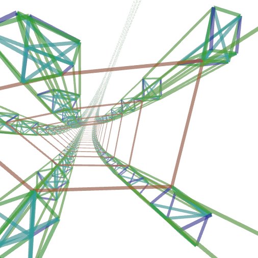
I am currently doing some research on procedurally generated 3D by inflating structures.

This blog post is about how the mathematics work.

Visualizing Infinite-Things-Space

Vertex data in a 3D structure is often stored in an array.
Ignoring the position and other attributes of vertices, each vertex can be represented as a natural number which refers to the index in the array of vertices.

To connect two vertices, I use a math formula that takes an index and outputs a new one.
The nice thing about this method is that you can compactly represent an infinite number of structures.

step1

When the function returns the same index, I visualize it as a loop for each natural number from 0 to infinity.

By adding by one, f(x) = x + 1, the loops are disconnect from themselves and attached to each other.

To create circles with 4 vertices, use the formula f(x) = x - x % 4 + (x+1) % 4.

Mathematical operations on the natural numbers are equivalent to operations on these loops.
For any mathematical expression of a single natural number, there is an equivalent shape in Infinite-Things-Space.

In group theory, these functions are called “generators”.

The Super Function

The Super function is a higher order function that takes a generator and produces a new generator. It preserves the structure of the input generator, but now “scaled up” with a factor of n.

super(n, f: N -> N) = \(x: N) = f(x / n) * n + x % n

The Super function is the key to combine multiple generators.

step2

f_0(x) = x - x % 4 + (x + 1) % 4
f_1(x) = super(4, \(x) = x + 1)

You can use the Super function with any generator, for example circles to create a donut topology (torus):

step3

f_0(x) = x - x % n + (x + 1) % n
f_1 = super(n, \(x) = x - x % m + (x + 1) % m)

When n and m in the example above goes to infinity, you can start at 0,
add infinity to take an infinitesimal step in the rotation direction of the torus.
Take an Aleph-1 step (a higher infinity), and you jump from the 0-point at the first torus
to the 0-point (modulus Aleph-1) to the second torus.

Inflating 3D structures

To inflate a 3D structure created by generators, I use an algorithm that takes a list of generators
and walks along all edges for a fixed range, generating a list of spring constraints.
If a generator leads back to the same vertex, it gets ignored.

The spring constraints are passed to a simulator that inserts random positions for vertices.
An extra spring constraint drives inflation by being connected temporarily between two random vertices A and B with a target distance 10 * (A - B).length().sqrt().

Inflation causes an internal pressure outward on the whole shape, so it unfolds into its “natural form”.

The square root operation is to avoid too much acceleration between distant points,
which might lead to stretching the shape like spaghetti.

Here is a shape inflated by connecting cubes with some internal support to edges of a pentagon,
which in turn is connected by a super hundredgon (a circle shape with 100 vertices).

torus

As you see in the picture above, the shapes do not become perfect.
This is because the springs are not possible to satisfy unless the differential topology is complete.
Because the inner circle is the same size as the outer one, the shape above twists and stretches the pentagons.

Finding a complete differential topology could be done by “tuning” the constraints while simulating,
or perhaps relaxing the target distances based on a function of the tension.
Alternatively, some new constraints could be added to keep edges at a fixed angle relative to each other.

The twisting effect can be used on purpose, e.g. on a cylinder with sinus modified distances:

twist

Have you seen how the sweets with double twisted paper get wrinkles? This seems to be the same effect!

Older Newer